Detecting and Mitigating Data Distribution Shift

Introduction

“Anyone who stops learning is old, whether at twenty or eighty. Anyone who keeps learning stays young.” - Henry Ford.

Can we say the same for our machine learned (ML) models ? In this post, I will share research that shows how models gets old or in other words, your data gets newer. I will also share techniques you can use to know when your model has become old (or your data has become younger) and how to refresh them without spending large amount of resources that you might have spent training them in the first place.

Data distribution shift also know as model degradation happens when a model does not perform as well on a dataset that is chronologically advanced than the dataset model was trained on. Model degradation is a misnomer in my opinion as the model did not really degrade, if you apply on similar distribution it will be great no matter what, rather its the data on which it is applied that has changed.

There are different types of drifts that a data can face any given time, however in reality they are all occurring on various scales simultaneously. Therefore, the more we can identify them to put checks and balances, the better we control the outcome of models in production. In the tree of types of drift, the three that sit at the top are label, covariate and concept shift. A label is category of your data that you’re trying to predict, covariates are features (predictors) that describe your data and concept is how the label is related to covariates in your given dataset. Let us understand these three shifts via a fun example.

Let’s say you train a model to differentiate apple and banana based a set of user buying patterns and it’s clear. You deploy it and it runs fine for a couple of months, until an article comes out which claims benefits of both are same and because apple is more expensive than banana, people that used to buy 🍎 have now started buying 🍌 instead. Consequently, this changes the relationship between covariates and the label itself hence leading to concept shift. Another type of shift called covariate shift, would be reduction is sales (used as feature in your model) of 🍌 Vs 🍎 because of an epidemic that causes 🐵’s to eat a lot more 🍌 leading to supply shortage. Lastly, in the same frame an example of label shift would that be over time (decades) farmers produce more of 🍏 apple than red 🍎, even though both are apples but the green one puts all work that went into selling red one out of window e.g. having to change brand color schemes or usage of fruit color as a feature in your model.

As we saw above, different factors can lead to different types of shifts. These factors range all the way from measurement noise, labeling noise, missing data, to environment change. While some are trivial to detect using well researched approaches, others like environment change are nuanced and hence difficult to detect. The field has sub-categorized these shifts further into following categories:

1. Anomaly detection: a data point is at least 2 standard deviation away from normal samples however even defining deviation for high dimensional datasets is hard.
2. Out of Domain: e.g. beer 🍺 classifier used as whiskey 🥃 classifier
3. Sub pop shift: in a multi-classification scenario, only some of the populations shift e.g. image based flower classifier performance degrades because a few classes of flowers evolved to have patterns with colors in petals that earlier were plain color.
4. Task shift: rare in industrial settings e.g. text sentiment analysis to entailment prediction

Shift detection is a fairly recent field that has emerged from the industrial applications of ML. Having model deployed in real-world created a need to have observability which is fundamental to how modern day software is deployed. This allowed teams to monitor how model is doing in production just like a software except the metrics changed. Because ML systems are rife with silent errors, their interpretation cannot be resolved by boolean logic. On the other hand, research came out that models especially neural networks do not generalize well to non-stationary data and are sensitive to even slight perturbations in data; in some cases even flipping the original prediction itself. This applies to pre-trained models as well (see work from DeepMind, Mohta et. al.). In Industry, this debt started affecting revenues as initial budget spent on training models went to waste when new data arrived and model could not perform the same. Lack of existing method combined with both of above factors created a sense of urgency that has led to development of new approaches for tackling shifts as well as adapting pre-existing models to new data.

Methods

Detecting shift

General ML

Seminal work by Rabanser et al showed that whenever a binomial test signals a statistically significant accuracy deviation from chance, it means drift has occurred. Further, they suggest monitoring the accuracy of models on examples on which it is most confident. In production, one can compare predictions on an inference set i.e. list of samples ordered by confidence by model with that of an expert, if the difference is statistically significant between held-out test set and inference set then there is drift. Note that this marginalizes sub-population drift by assuming number of samples in test set would be large enough. This technique is the simplest method one can add to their production stack to detect drift, however has drawbacks biggest one being large number of false alarms e.g. accuracy is down by 5% in the past hour, could mean incoming data is different temporarily which means drift or frequency of a subpopulation increased in the time frame in which model accuracy historically has been 5% less which makes it a false alarm, etc. Recent ICLR 2022 paper by Davari et. al. also showed that model can maintain task accuracy with degraded representations as well.

Having confidence intervals (CI) around your point estimates (predictions) helps instill confidence in your team when putting a model out there. CI provides a range of certainty within which the predicted probability lies, the tighter the CI the lower margin for error and vice versa. Bayesian inference provides CI out-of-box[1] however is computationally hard to do, hence most of ML relies on discriminative models that can only provide point estimates. This urged practitioners to come up with techniques that even though remains in discriminative realm but still provides prediction intervals.

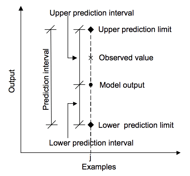
A common method for generating CI is bootstrapping, which is sampling a subset with replacement. This technique was devised in 1979 by Brain Efron, and is one the most helpful tool in an MLOps arsenal. By bootstrapping multiple subsets of a held-out test set and recording performance metrics (e.g. accuracy) on it, one can then get a distribution of metrics and compute a 95% CI on it. Users should take into account the time frame to make realistic estimates e.g. if your business team cares about metrics no less than 2 weeks time frame then no point, on the opposite even if your team cares in 2 weeks but number of samples per bootstrap aren’t enough then you need to increase time window to gather more samples. At inference, if prediction is outside your CI then you can flag it for review.

There has been an another emerging field of conformal prediction to build intervals around our predictions not only of point estimates but sets. It builds on the concept of trusting samples that a model has seen before more than that of unseen. It can happen in two ways, either using confidence from model (1 — the predicted probability) or the ratio of distance from training samples of a given class from different classes. Therefore, providing not only confidence but also credibility. Credibility measures how likely the sample is to come from the train set, this is given by the minimal significance level such that the conformal region is empty. It does so fundamentally by measuring confusion of a classifier i.e. if a model gives high probability to multiple classes or reverse giving low probability to multiple classes. The technique can be extended to a clustering based approach where equidistance to cluster centroids can be seen as a source of confusion.

Methods based on point estimates can only go so far, in cases where you have access to model itself or maybe even have control over its training procedure, we can do better. UQ in neural networks starts with either removing some connections between nodes or zeroing arbitrary node with some probability or a hybrid of both, most famous of them being Monte Carlo (MD) dropout. At inference, the process would be repeated multiple times to build a CI. Even though MC dropouts are agnostic to drift changes and lie in same category as prediction interval techniques. There is one technique that has been found to be robust in OoD generalization called ensembling. Deep ensembles are created by training a neural network model with different random initialization that leads to model learning different aspects of data.

In cases where we have access to both training data and trained model, several techniques compare encoding of training data with that of an inference set using a distance metrics. These metrics can help provide an estimate of how likely is the inference set coming from the same distribution as training set w.r.t. model parameters. Because training set is large, doing two-sample statistical tests would be costly and would only take us so far in high dimensional problems, instead we can compare mean encoding of training set with that of an inference set. A standard metric for that is Maximum Mean Discrepancy (MMD) which is the squared distance between two means. MMD however comes with high computation cost and does not offer nice properties of two-sample tests for anomaly detection, therefore a recent work proposed a partial-Wasserstein distance (also known as Earth Movers Distance in optimal transport literature) instead which bridges the gap between drift check and anomaly detection. Authors also proposed an approximation of MMD named partial-MMD that is relatively cheaper to compute and has equivalent performance.

Another clustering based technique is to create a distribution of distances of samples for each class from their cluster centroids. At test time, a two sample distribution test of the distance of sample for the predicted class can be used to decide if sample belongs to cluster. The two sample tests depends on outcome variable such as Kolmogorov–Smirnov for continuous distributions, Statistical Process Control methods for rate of change, Chi-squared for 0-1 or pre-defined margin e.g.alert if predicted probability is between 0.45 and 0.55. The idea of MMD can be extended and if predicted class is with high confidence then cluster membership can be resolved by a MMD between cluster and inference set.

Having access to model weights and training data allows us to further analyze the manifold. Several works have explored empirically identifying the dimensions that are susceptible to shift. This is done by measuring extent of degradation in performance along a particular category of data one at a time. The categories that degrade the performance reveal drawbacks in the model. The model can then be adapted to these sensitive categories to make it more robust and hence reduce susceptibility to drift.

So far we’ve seen approaches that are general enough to be applied to any ML application depending on access to prediction probability, model weights, control over training and training set itself. Furthermore, if we know the domain of application we can use methods that are specific to the domain and lead to improvements. Let us review the techniques for the two most prominent applications of ML today namely Computer Vision and Natural Language Processing (NLP).

Computer Vision

Much earlier than NLP and stable. Has overlap with corruptions handling or increasing robustness of the models. It also shares work with research in algorithmic scene change detection. The primary contributors to data shift in real-world applications can be anywhere from camera noise, dynamic adjustments of the camera parameters (e.g. auto-exposure, auto-gain) to global (e.g. a cloud passing by the sun, light switches) and local (e.g. shadows cast by moving objects, light spots) scene illumination changes.

Similar to how perplexity of an inference set was compared to baseline perplexity on test set in NLP, over on the CV side instead of perplexity, reconstruction loss is used.

This loss is computed as follows:

1. An encoder-decoder setup is used where model is tasked with encoding image into latent space which is used by decoder to recreate the image.
2. To measure how successful the recreation is, a re-construction loss is used. This loss is recorded on a held-out test set and a distribution is built or a threshold is used to identify anomalous data.
3. At inference, two sample test or threshold is used to identify samples a model is un-sure about.

Since measurement noise and robustness to it plays a crucial role in CV, we also setup auxiliary tasks to identify the type of noise itself. The other method would be recording metadata embedded in images (camera type, geo tag, resolution, etc) from EXIF/TIFF tags or computed from it like HSB (hue, saturation, brightness) and comparing it at inference to flag anomalous samples.

While most of the noise can be eye-balled, there is a type of noise that bypasses human eye but affects models drastically. Seminal paper by … took the CV world by storm that showed an image can be modified in ways that changes model behavior but is indistinguishable to human eyes. Eversince then, tremendous work has gone into making models robust against noise like this especially in production. Initial works proposed using constrained noise sampled during training, however that came with guesswork of identifying noise types beforehand which is hard to do. The prominent among them is adversarial adaption which introduces noise that model defaults on as one of the labels and the updates model by teaching it to account for the adversarial noise as well. For details on different types of attacks and countermeasures, refer to survey by Akhtar et al.

NLP

Shift detection in NLP evolved from diachronic linguistics where early works traced changes in frequency distribution of vocabulary of a corpus over time using models from the field of diffusion theory. Some methods also use the contribution of Shapley values to final prediction as a means of tracking shift i.e. when there is a drastic (two-sample test) change between two time spans, then shift has occurred. While earlier approaches compared statistics of corpus, later work used cosine similarity of the encoding of the trained model for corpus over time to study shift. With the advent of word embeddings circa 2015, changes in the distributed representations of the words started being used to track changes in meaning of words over time. MMD of inference set from mean encoding of training set could be used to detect shift. Techniques that computationally study evolution of language worked well until arrival of Large Language Models (LLMs) having billions of parameters, making it infeasible for most researchers to apply previous methods, therefore, new methods had to be devised.

Work from DeepMind studied LLMs temporal generalization with the lens of perplexity. Perplexity is the negative log likelihood metric used to measure quality of a language model that avoids bias due from sequence length. They find that model performance becomes increasingly worse with time. This is built on work of Lee et. al. who show that misinformation has high perplexity. Therefore, similar to two sample hypothesis testing, one could compare validation set perplexity with that of incoming sample, if it’s outside 95% CI then it could be flagged. This intuitively means the model is more confused on inference that it is on training set implying shift.

Recently, Arora et al has categorized OoD texts into either of background or semantic shifts. Background means change in style independent of the label e.g. style, domain, genre of text while semantic means change in meaning of the discriminative features themselves i.e. dependent on the label. Furthermore, they also find that it entirely depends on the use-case which among the two main types of OOD detection methodology is best. Therefore, authors prescribe doing due diligence on the anticipated shift type in production and accordingly using appropriate technique.

Above methods are useful for nuance shift detection, but a robust anomaly detection pipeline precedes it all. For NLP it would mean setting alerts of text length, repeated sequences, etc while for CV it would be all black / white image, large area of occluded, etc.

Speech

Once transcribed gets reduced to text, it becomes an NLP problem to which all techniques we covered in previous sections can be applied. However, even before transcription a model can face all sorts of shifts e.g. Speech decoding model trained on US accents gets deployed in Africa would fail miserably due difference in accent. Most the the techniques covered under domain adaptation can be used to address shift in speech data. We’ll cover techniques specific to speech in a future post.

Mitigating model staleness

There are several way to approach fixing model staleness depending on how much access one has to the ML life-cycle. Calibration methods are used when you only have access to model predictions, while density estimation methods are more involved with their usage of model internals and datasets. Naturally, density methods provide better robustness as you can explore and adapt your model to new tasks or shifted datasets. Calibration relies on using threshold of prediction and Density estimation instead fits model to a distribution. A middle ground can also be had by training surrogate models that learn to identify how a base model makes mistakes and corrects or flags them in production. Let us look at each of them in detail.

Calibration

This method relies only on the predicted probabilities and sometimes labels of train, test set. This comes with numerous of advantages such as no assumption on type of models, light weight by not needing access to datasets and consequently easy to implement. At the heart of this, a regression is performed that maps probabilities of original model to that of shifted data e.g. mean and variance of a feature in data shifted by 10%, then weightage is increased. Another method is to use thresholds, metrics are recorded and sorted followed by finding a threshold that allows pre-decided error rate. At test time, if threshold is crossed then an alert is triggered. If threshold is crossed for large number of samples All of these techniques can be used to learn weights that adapt output of model to newer datasets.

Traditionally platt and recently temperature scaling has been used as a method to learn scaling weights on new dataset. However, platt’s advantage of being able to work on small datasets comes from its assumption about the use of Gaussian distribution which can become its achilles heel. Further, another type of calibration named Isotonic regression learns a mapping by fitting a logistic regression or finding least squares estimates to classifier scores. To improve, beta calibration was proposed which does not make any implicit assumptions about the distributions. These worked well for non-probabilistic estimators however fails when data is low (overfitting) or function is not monotonically increasing. Kumar et al recently found out that calibrating on in-domain surprisingly improves the OoD accuracy of the ensemble of standard classifier and robust (spurious correlations removed) classifier.

A different approach was recently proposed namely Average Threshold Confidence (ATC). ATC finds a threshold on validation set such that the fraction of samples that receive the score above a particular threshold match the accuracy of those samples. This guarantees the performance in inference set in-turn controlling cumulative error rate of the classifier. Recently, Guillory et. al. in Predicting with Confidence on Unseen Distributions found difference of confidences (DoC) to be better than ATC (reduced error in half compared to ATC) and even MMD in some cases. DoC is calculated by taking batches of held out test sets and measure how much do their confidences vary. While this does not directly adapt the model, it helps control the accuracy a model achieves and hence adapting it to fresher datasets.

Even though calibration is helpful in that it is lightweight (not needing access to model weights or retraining), this itself becomes its achilles heel. Calibration methods fails when a trained model relies on spurious correlations for prediction. OoD data would also comprise of same correlations regardless of unseen domain hence would result in false alarms. Mohta et al also showed performance drops when domain of pre-training and fine-tuning are not similar. Davari et. al. also found that continual learning under breaks distribution shift.

Density estimation

Unsupervised domain adaptation aims to learn a prediction model that generalizes well on a target domain given labeled source data and unlabeled target data. Some works simulate drift when training model itself. Kong et al propose methods for calibrated language model fine-tuning for in- and out-of-distribution data. Mohta et. al. study the impact of domain shift on the calibration of fine-tuned models. They find the pre-training does not help when fine-tuning task has a domain shift.

Shen et al shows how contrastive pre-training connects disparate domains but should only be used when one anticipates facing drastic out of domain in production. They show that extra unlabeled data improves contrastive pre-training for domain adaptation. This is especially important in vision domain where a camera change might introduce a shift that the model can adapt to.

In cases where models are deployed on the edge, test time adaptation to shifts becomes crucial. Teja et al instead propose that if a model’s predictions is consistent with some margin to augmented data then it will increase robustness when drift occurs. Recent work by Wu et al proposed fine-tuning with auxiliary data. My recent paper proposed a method named MEMO-CL for improving adaptation of large language models by minimizing entropy of output distribution on a batch of synthetic samples conditioned on a test sample. Other works reduce variance by augmenting data during training process. This post from Lilian Weng has nice overview on data augmentation methods.

Domain adaptation / Adversarial approaches makes implicit assumptions about the OoD distribution or learns to make model robust on gaps created in representation of training dataset itself. This is sub-optimal as in real-world setting, often there is less control on how new form of dataset emerges. Furthermore, this approach comes with the trade-offs in performance as we’re trying to be as generalized as possible. Therefore, a better option would to learn to abstain from predicting if model is not confident enough, this allows us to control for risky cases where cost of false positive would be high. Zhang et al propose hybrid models for open set recognition i.e. identifying cases. Liu et al propose hybrid discriminative-generative training via contrastive learning. Both of these models try to recognize training set from data in any other distribution.

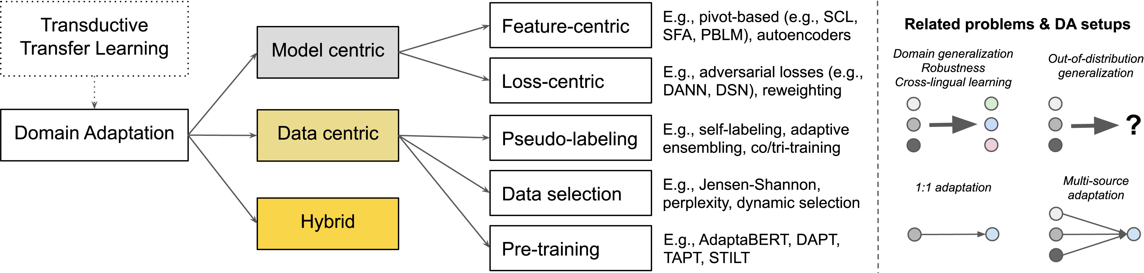
There are other emerging methods such as self-supervised and contrastive DA that attempt to leverage given data itself or seeks unlabelled sources to gain further signal. This can come in the form of generating pseudo-labels, tasking model to predict part of the masked data, new loss functions, or selecting the right data points. Survey done by Ramponi et. al. covers in detail different techniques that have been proposed in the recent past.

Practitioner’s Checklist

I have divided the approaches one can take to address distribution shift based on which stage of the ML life-cycle you’re on.

Pre-training

1. Find optimal time window to build reference dataset to be tested for drift. This will use useful in creating 1) calibration and 2) inference set.
2. Carve out a calibration set that is separate from held-out test set and to be used after evaluating on test set first.
3. Pay attention to
   1. the type of split, prefer chronological over random as its more representative of recent data which gives you a better estimate w.r.t. drift.
   2. maintaining i.i.d. and temporally stratified sampling
4. If possible, try to identify the type of shift you’ll most likely to experience between background or semantic.

In-training

1. Open Set Recognition: Learning to abstain from prediction by differentiating in from out-of-domain distribution during more training
2. Dropout to increase generalization and get uncertainty during inference
3. Train Ensembles if you can afford, if you cannot or are fine-tuning then doing ensembles of the last layer would still be better than nothing.
4. Don’t throw away your checkpoints: they’re free ensembles and we know that deep ensembles are one of the most robust methods against shift.
5. Build invariances into your models: via data-aug and domain-adaptation technique

Post-training

1. Calibration
2. MSP baselines (even better MLS)
3. ATC / DoC baselines
4. Conformal prediction
5. Clustering

Post-deployment

1. Statistical testing on average metric degradation e.g. probability, accuracy of a batch
2. Use MSP baseline calculated post-training to mark mis-classified or out of domain samples.
3. MMD or Wasserstein (EMD) distance check (not KL as it’s not symmetric) between mean training set and inference set encoding. The inference set is created using optimal time-window calculated in pre-training phase.

4. Rely on adaptation techniques i.e. continual pre-training (not fine-tune) which comes free. Use a separate VM to adapt OR get creative with your usages e.g. re-use the same machine you have for production to train.

   Keep in mind that mitigation comes with its own can of worms, the biggest one being catastrophic forgetting. Remember, the biggest challenge back in 2016 with trying to do transfer learning was catastrophic forgetting, which happens when a model forgets it’s priors or in other words forgets what it had learned during training from original data when trained on a new dataset. Quite a lot of research has gone into trying to avoid it like removing lower layers, using smaller learning rate, distillation until LLMs came along that even though showed signs of catastrophic forgetting but to a smaller extent.5

5. Cluster assignment testing: keep tabs on how easily can a given test sample be assigned a cluster. This will not scale if the data high dimensional.

Datasets

Oftentimes, it’s hard to collect data that is naturally labelled in order to study shift patterns in private datasets. For times like these, along with having novel techniques as we saw above it is also helpful to have some gold standard datasets on which you can test your methods on. Here a few datasets you can test your models on for drift.

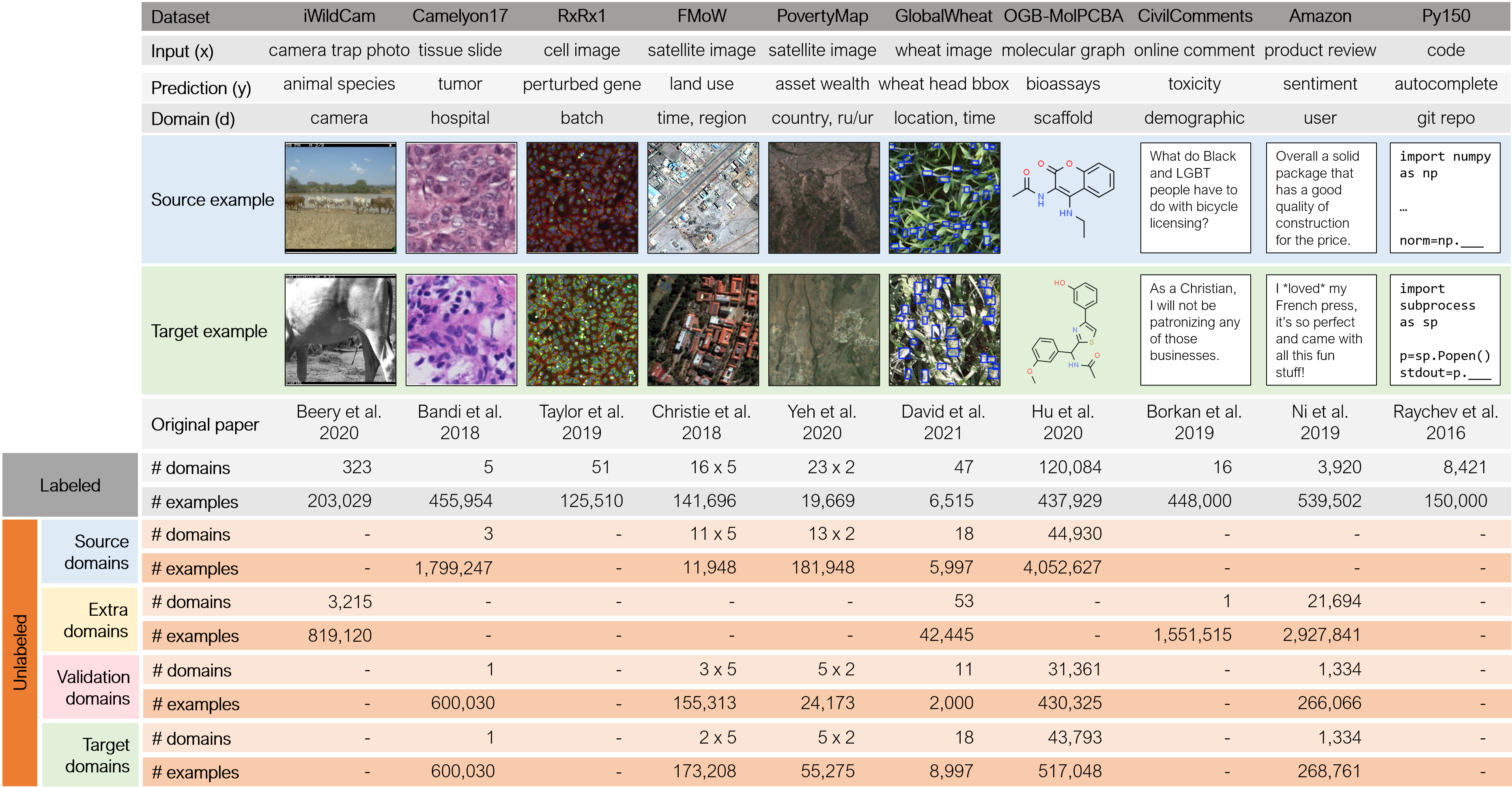
Sagawa et al introduced WILDS is curated collection of datasets from different domains ranging from images, biomedical graphs to product reviews. The goal of WILDS is to allow researchers to test both OoD and sub-population shift generalization. An extension of WILDS with curated unsupervised examples was also introduced recently. These datasets span a wide range of applications (from histology to wildlife conservation), tasks (classification, regression, and detection), and modalities (photos, satellite images, microscope slides, text, molecular graphs)

NLP datasets

For natural language processing, shift is much harder to detect compared to vision e.g. shift in intensity of argument Vs. corrupt pixels or occlusion (ignoring adversarial image corruption).

1. Twitter streams: for studying diachronic shifts. Work has been done to also leverage metadata mentioned by users in their profile bio to study how different regions expression of language evolves over time. This data can be used to study both temporal generalization and out of domain.
2. WILDS-Civil Comments: toxic detection for OoD detection
3. WILDS-Amazon: 233 million amazon product reviews timestamped between 1996 - 2018.
4. BREEDS: assess robustness to subpopulation shifts, in particular, to understand how accuracy estimation methods behave when novel subpopulations not observed during training are introduced.
5. WMT News Crawl: collection of news articles timestamped with year of publication from 2007 - 2021.
6. arXiv: highly granular timestamped collection of scientific abstracts along with metadata on various domains like physics, maths and computer science.

CV datasets

Similar to NLP, in and out-domain datasets can be easily created by training on dataset from one domain and applying on other. Note that for iWildCam and FMoW in WILDS, recent work has found 1) weak correlations between validation and test set 2) high correlation between some domains 3) baselines being sensitive to hyper-parameters 4) cross-validation is crucial when working with these datasets. Other datasets exists suchs as Landscape Pictures and IEEE Signal Processing Society Camera Model Identification

For simulating semantic and subpopulation drift, one can use CIFAR-10 or ImageNet to hold-out some of the child classes e.g. hold out trucks while train on cars, both come in automobile category or hold out horse and train on deer.

For those working on graph datasets, recent work introduced GDS , a benchmark of eight datasets reflecting a diverse range of distribution shifts across graphs.

Other techniques

If one has access to structured metadata of dataset, it can be used to create OoD like that of WILDS data where some categories can be held out, while others can be used to train a model. For example, if demographic is known in a sentiment classification model then OoD can be created stratified by state, this will reveal performance of model trained on data for some sets when applied to other states. This can happen in real-life where business team once confident on a model on a certain population will want to use the same model for other populations as well. Repeating this method for different categories in a dataset can surface problems in data, model architecture, sampling bias, etc.

Another type of data that has gained popularity in recent times in Counter-factually Augmented Data (CAD). This type of data is created manually where experts are asked to change the input just enough to flip the polarity for example in a sentiment classification model. There have been that used distant supervision combined with templates to generate this type of data. Kaushik et al c-IMDB Learning the difference that makes A difference with counterfactually augmented data. Sen el. al. use CAD data to study model’s dependency on sensitive features in How Does Counterfactually Augmented Data Impact Models for Social Computing Constructs? Their data generation methods can be leveraged by teams to generate their own versions, a combination of TextAttack, NLP behavioral checklist, gender, sexist, and hate list.

Data Preparation

Chronological split

This type of split entails that most recent data point in your training set be earlier than earliest data point in your test set. Similarly, validation / dev set data points fall between train and test set.

Out of domain

A common method of testing OoD generalization is used to stratify using some metadata column to keep part of data in-domain and leave the rest for testing making it test set belong to OoD.

Splitting methodology matters

Sögaard et. al. show that the standard random splitting over-estimates performance. Similar effects are observed when data is not chronologically split i.e. training data does not precede test data. Often times business stakeholders can guide you in deciding the split itself e.g. medical knowledge updates every 73 days, therefore the guidelines used for decision making also changes to varying degrees. More often than not, splitting your data chronologically will provide realistic estimates rather than random. If you have low data, prefer cross validation or if you have high budget then evaluate both on random split as well as chronological split.

SimplerOne can also go as far as to generate an optimal split by finding points that maximize Wasserstein distance between clusters created from a validation set.

Preprocessing

This can take a post of it’s own, but at the very least users should strive to make sure data is i.i.d. which is not easy to do when aiming to nullify auto-correlation. Secondly, deduplication can be useful as data generation process often times introduce similar articles e.g. article posted on NYT today, an excerpt posted few months after, then year later it becomes relevant to everyone is writing versions of it.

Note on avoiding data leakage: Although hard to do, de-duplication between articles published that share same set of subjects over time e.g period of presidency will have news of a particular person, it can also double down as as OoD task when model learned from articles of one president can be used to evaluate on other president.

Libraries

Thanks to open source community, there are several libraries that help detect drift. The most popular and stable among all is alibi-detect which also supports outlier-detection. It primarily uses MMD which is one the best methods out there, but what I find even better is they have an expanding window approach that reduces false alarms. To elaborate, we don’t know how many samples we need in inference set beforehand when computing MMD, too low and it goes undetected and too high it increase false alerts. Therefore, alibi-detect starts with a small window, if there is a slight signal of drift happening then it increases window to gain more samples in-turn increasing statistical significance. That way, it only alerts when it has gained enough confidence that there is indeed a drift not a fluke.

For deep-learning, torchdrift.org recently came out, the tensorflow world has it’s own TF validation module that allows developers to do define constraints, however its more focused on validation rather than drift detection. Some cloud vendors like AWS (SageMaker) and Domino also offer this out of box, although I have not tried either of them I feel like they’re more like TF validation than alibi-detect.

Adversarial evaluation is great at pinpointing gaps in model. For CV, cleverhans and for NLP TextAttack and nlpaug are great that can be combined with NLP behavioral checklist. Finally, adversarial-robustness-toolbox tilts more towards securing your models in production against attacks. These libraries make it easy for practitioners to cover more ground when it comes to successfully putting models in production.

Apart from using libraries for detection, there are libraries available that will allow one to surface problems in their models like bias. If you have demographical metadata, you can use fairlens library to evaluate whether your models are fair or not.

Summary

Hopefully by now you have enough context on the state of techniques at your disposal for alleviating distribution shifts and take measures to prepare your models in advance for when shift happens.

When it comes to adaptation, it is advised to do some due diligence on the type of problem and environment where your models will be deployed to get an idea of type of shifts. As showed by Wiles et al after doing 85,000 experiments on numerous datasets and techniques to address shift, it was found that techniques like pre-training and augmentation do help mitigate staleness, the best methods still are not consistent over different datasets and shifts.

Feel free to come back to above mentioned practitioners checklist. I also gave a talk on the subject recently which goes over some aspects like open set recognition as well.

Appendix

Examples

A collection of examples that can help understand the concept better.

In an effort to reduce bias towards British expression of language, say an erroneous GEC system is introduced by Google which lets one write colour as color or analyse as analyze. Now your statistically trained LLM has seen alot of one but not the other, even though semantic meaning p(y|x) remains the covariates (input) distribution has shifted p(x).

MLOps

If you’re interested more in MLOps side of things, Chip Huyen wrote a comprehensive article on Data Distribution shifts and Monitoring. Her work focus on things from overall perspective because of which there is less emphasis on how to actually go about detecting and fixing shift. This inspired me to write my own version that is more inclined towards modeling.

References

1. Kendall, A., & Gal, Y. (2017). What uncertainties do we need in bayesian deep learning for computer vision?. Advances in neural information processing systems, 30.
2. Gama, Joao; Zliobait, Indre; Bifet, Albert; Pechenizkiy, Mykola; and Bouchachia, Abdelhamid. “A Survey on Concept Drift Adaptation” ACM Computing Survey Volume 1, Article 1 (January 2013)
3. A. Ramponi and B. Plank, “Neural Unsupervised Domain Adaptation in NLP—A Survey,” in Proceedings of the 28th International Conference on Computational Linguistics, Barcelona, Spain (Online), Dec. 2020, pp. 6838–6855. doi: 10.18653/v1/2020.coling-main.603.
4. J. Choi, M. Jeong, T. Kim, and C. Kim, “Pseudo-Labeling Curriculum for Unsupervised Domain Adaptation.” arXiv, Aug. 01, 2019. doi: 10.48550/arXiv.1908.00262.
5. X. Ma, P. Xu, Z. Wang, R. Nallapati, and B. Xiang, “Domain Adaptation with BERT-based Domain Classification and Data Selection,” in Proceedings of the 2nd Workshop on Deep Learning Approaches for Low-Resource NLP (DeepLo 2019), Hong Kong, China, Nov. 2019, pp. 76–83. doi: 10.18653/v1/D19-6109.
6. A. Cossu, T. Tuytelaars, A. Carta, L. C. Passaro, V. Lomonaco, and D. Bacciu, “Continual Pre-Training Mitigates Forgetting in Language and Vision,” ArXiv, 2022, doi: 10.48550/arXiv.2205.09357.
7. X. Jin et al., “Lifelong Pretraining: Continually Adapting Language Models to Emerging Corpora,” in Proceedings of BigScience Episode #5 – Workshop on Challenges & Perspectives in Creating Large Language Models, virtual+Dublin, May 2022, pp. 1–16. doi: 10.18653/v1/2022.bigscience-1.1.
8. A. Machireddy, R. Krishnan, N. Ahuja, and O. Tickoo, “Continual Active Adaptation to Evolving Distributional Shifts,” in 2022 IEEE/CVF Conference on Computer Vision and Pattern Recognition Workshops (CVPRW), Jun. 2022, pp. 3443–3449. doi: 10.1109/CVPRW56347.2022.00388.
9. D. Kim, K. Wang, S. Sclaroff, and K. Saenko, “A Broad Study of Pre-training for Domain Generalization and Adaptation.” arXiv, Jul. 20, 2022. doi: 10.48550/arXiv.2203.11819.
10. S. Garg, S. Balakrishnan, and Z. C. Lipton, “Domain Adaptation under Open Set Label Shift.” arXiv, Jul. 26, 2022. doi: 10.48550/arXiv.2207.13048.
11. X. Dong, L. Shao, and S. Liao, “Pseudo-Labeling Based Practical Semi-Supervised Meta-Training for Few-Shot Learning.” arXiv, Jul. 14, 2022. doi: 10.48550/arXiv.2207.06817.
12. K. Shen, R. M. Jones, A. Kumar, S. M. Xie, and P. Liang, “How Does Contrastive Pre-training Connect Disparate Domains?,” presented at the NeurIPS 2021 Workshop on Distribution Shifts: Connecting Methods and Applications, Dec. 2021. Accessed: Sep. 06, 2022. [Online]. Available: https://openreview.net/forum?id=ZKCw3atVfsy
13. M. Davari and E. Belilovsky, “Probing Representation Forgetting in Continual Learning,” presented at the NeurIPS 2021 Workshop on Distribution Shifts: Connecting Methods and Applications, Dec. 2021. Accessed: Sep. 04, 2022. [Online]. Available: https://openreview.net/forum?id=YzAZmjJ-4fL
14. S. Mishra, K. Saenko, and V. Saligrama, “Surprisingly Simple Semi-Supervised Domain Adaptation with Pretraining and Consistency,” presented at the NeurIPS 2021 Workshop on Distribution Shifts: Connecting Methods and Applications, Nov. 2021. Accessed: Sep. 13, 2022. [Online]. Available: https://openreview.net/forum?id=sqBIm0Irju7
15. A. Singh and J. E. Ortega, “Addressing Distribution Shift at Test Time in Pre-trained Language Models,” Dec. 2022, doi: 10.48550/arXiv.2212.02384.